DEFINING ELECTROFACIES: SUPERVISED AND NON-SUPERVISED APPROACES
Multi-variate statistics provide the right tools that allow:
o to analyze wireline logs and core data;
o to predict electrofacies from a large number of wells and using complete sets of logs;
o to calibrate the detected log facies against core data;
o to predict the bog facies at the non-cored intervals and non-cored wells;
o to quantify the uncertainty of the bog facies determination.
A non-supervised approach, is purely based on multi-variate statistical analysis of the wireline logs, regardless of the core data.
A supervised approach, integrates wireline logs with core data.
These two basic approaches can be combined to identify and predict optimal log facies at cored and non-cored wells, in an integrated and robust workflow:
o Multi-variate density function interpretation and cluster identification
o Cluster interpretation and electrofacies definition, using core data
o Electrofacies prediction at the non-cored intervals of non-cored wells.
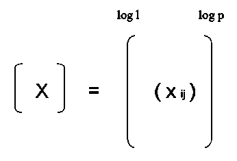
Well data are a set of z values. A Set of log measurements is associated to each z value. Data can be represented as follows:

Matrix of the data
( x ij ) = log j measurement at the point i .
An electrofacies is nothing but a cluster of z values in the space. Its geological meaning is a priori known or it must be interpreted (from core data for instance).
The electrofacies gathering depends closely on the variables (logs) in use. The electrofacies definition and prediction normally
combines a statistical analysis with the standard geological interpretation of logs. Logs and core data are both taken into account in order to generate facies logs that honor both pieces of information.
Two different classification methods can be performed: a supervised and a non supervised. The supervised approach takes into account a priori data given by the geologist which constitute the " training sample ".
The number of classes and their log characteristics are determined by these data. When running a non supervised approach, the training samples are defined from the interpretation of the density function calculated on log data. The number of classes and the corresponding characteristic samples are decided and selected at this step. Their geological meaning will be interpreted from their location in crossplots and from core data.
The two methods can be run independently or be linked together:
o electrofacies detected during a non supervised approach can constitute a training population to add as a priori information to a supervised study;
o the geologist can add an a priori supplementary class to these that have been interpreted during the non supervised approach.
The non supervised approach
The non supervised approach can be divided into 3 important steps.
o density fünction estimation,
o density function interpretation: number of classes, creation of the training sample,
o data points assignment.
Density function estimation
An electrofacies is nothing but a gathering of points together in the log hyperspace. Electrofacies classes constitute a set of points separated by areas with low density of points. By detecting and analyzing the variation ofthe density in the log hyperspace, it is possible to detect these different sets. The number of density peaks defines the number of classes. Points highlighted in these zones of high density correspond to the most typical samples of each dass.
The probability density function (PDF) describes the distribution of a variable and gives its associated probabilities. In a univariate case, the PDF is often described in a discrete manner with an histogram. However this histogram is not a good density function estimator. lt does not give the number of samples for a particular value; it only gives the number of samples that fall into an interval.
In a p-dimension space (corresponding to the p logs which are used), the PDF is estimated using KNN (K nearest neighbors) or kernel techniques (Gaussian, Epanechnikov, etc.). If only one variable is used, the density function is a curve (that can be approximated by smoothing a histogram). If two variables are used, the density function is a surface with valleys and hills like a topographic surface. When more variables are used, it is not possible to represent the PDF, however, we can analyze the peaks ofthe PDF using Kittler algorithm. This technique is called the mapping of the PDF or PDF mode mapping :
o A random point is chosen.
o A neighboring is defined in order to calculate the slope in all directions.
o The next point is chosen from nearby in order to move as far uphill on the PDF as possible (i.e. the greatest slope is used)
o The process goes on until reaching a density peak.
o From this, the following points are selected in order to ensure that one moves as little downhill as possible until a minimum of the PDF.
This gives a path that climbs steeply uphill to a mode and then goes down slowly, visiting all points. The neighboring, called " Mode mapping parameter"‚ is the smoothing parameter to choose.
If it is too big, you loose information about density. if it is too small, all the details are mapped, even the small ones, introducing
noise in the Interpretation.
Assignment of samples to a class: the classification method
The next step of the classification aims at classifying all log samples.
At this point statistical techniques such as discriminant analysis or pattern recognition can be used. In the methodology presented in this paper, the discriminant analysis is used. lt is fast, robust and has shown an unmatched efficiency and reliability on any type of environment (clastics and carbonates).
In a discriminant analysis, the probability of belonging to a class is computed for each sample. The point is next allocated to its most probable belonging class. This calculation uses the well-known Bayes formula. Various kinds of discriminant functions can be used for classifing the samples:
o The linear hypothesis: the covariance of each class is assumed to be the same,
o The quadratic hypothesis: for each class a distinct covariance is calculated from the training sample.
o Non-parametric hypotheses can also be made.
In such a case, the probability laws for each class have to be estimated using Kernel or K Nearest Neighbors methods. These laws are nothing but the PDF of each class.
Obviously, the less hypothesis on the model is assumed, the more closer we are to the reality. Ideally, the non parametric approach is the most promising, but with this approach, we need a lot of points in the training sample to obtain a reliable result.
Once the assignment method is chosen, the training samples are stored as non allocated points. The method efficiency can be evaluated by computing the percentage of well assigned samples (i.e. which are allocated to their actual class).
This method anyway underestimates the error rate because observations to evaluate die classification results are the same to build the classification rules.
For this reason, a second series of validations is carried out. A sample is taken out of the training sample before building the classification rules.
It is re-allocated using this rule afterward. This is a more pessimistic but realistic measure of the classification efficiency .
Quadratic and linear hypothesis give good results. Cross validation is interesting, in the linear and quadratic case, only if the number of points is not too large. Otherwise, if you remove a sample from a lot of points, it has a little impact on statistical methods using only mean and covariance matrices. However, in a non parametric case, this diagram is always interesting to be consulted because removing even one point could affect intra-class density estimations.
Supervised approach
In a supervised approach, we have an a priori training sample coming from a geologist prior interpretation. The number of classes is given, it is a part of the geological a priori. The classification function is created from this a priori training sample. All the points will be assigned to a dass using this classification function.
Everything is known since we have already discussed the discriminant analysis in the frame of the non supervised interpretation: we have to choose the hypothesis (linear, quadratic or non parametric), in order to run the classification and check the results.