www.GeoNeurale.com
NEWSLETTER CONTENT
GeoNeurale
Courses Program 2008
Double Duty with The Old and The New (by Gene Ballay)
BibliograpyCarbonate
Petrophysics Consulting
References
and Links
DOUBLE
DUTY with THE OLD and THE NEW
by
R.E. (Gene) Ballay PhD
Abstract
It
seems like only yesterday that I reported to work at Shell’s Bellaire Research
Center. Gus Archie was already gone but Monroe Waxman (Waxman-Smit’s equation),
Bob Purcell (developed mercury injection capillary pressure), Jerry Lucia (Rock-Fabric
Carbonate Pore Classification) and many other fine professionals were always
willing to take time to explain their trail-breaking work to a neophyte.
In
those pre-computer days (Schlumberger’s CSU truck was not yet operational),
petrophysical evaluations were, by necessity, very different than today. And yet
with skill, insight and experience, petrophysicists such as Lou McPherson (who
ran Shell’s Petrophysics Training Program) were able to evaluate intervals
that, even today, would challenge the computer.
Computer
interpretations, deterministic and probabilistic,
typically place many
evaluation options at our disposal,
and are without doubt a major step forward. Unfortunately, in an era where
animated power point slides are the norm, it’s
also possible to over-look fundamental, under-lying petrophysical concepts that
remain valid, whether applied with log-log graph paper or the latest
probabilistic software.
Bulk Volume Water
The
surface to volume ratio of a sphere is (4 p r 2 ) / (4 p r 3
/ 3 ) ~ 1 / r . This relation reveals that pore
surface area becomes a relatively larger issue, as the pore radii decreases
(1 / r increases). In the case of water
wet rock at some
specific height above the free water level, one then anticipates
an increased Sw, as pore size decreases.
Archie,
who was in fact far more than Archie’s equation, documented
this
relation in his 1952
publication (Classification of Carbonate Reservoir Rocks and Petrophysical
Considerations) with a graphical display of Porosity vs Water Saturation.
With
Porosity along the vertical axis and Water Saturation plotted horizontally, Archie
found that discrete pore sizes trended along approximately hyperbolic lines of
roughly constant product value
(ie Porosity * Water Saturation = Constant): Figure 1. Larger pores corresponded
to lower constants, because the (water wet) surface area / volume ratio
decreased.
FIG. 1A
| FIG. 1
Bulk Volume
Water
•Reservoir
performance can often be evaluated in terms of the Bulk Volume
Water
BVW = Sw * Phi
•Contour
lines of constant bulk volume water may be used as cut-off
boundaries
•Permeability
estimates may also be possible in favorable situations
•The
graphic consists of Water Saturation versus Porosity. Depending
upon local conventions, either
attribute (porosity
or water saturation)
may be along the vertical axis, with the other being along the
horizontal
•In
the Log-Log
world
(such as used in a Pickett Plot), these BVW
trends are straight lines
|
Roberto Aguilera remembers G. R. Pickett as a true Giant and a great professor of petrophysics. He always tried to teach us to stay away from what he used to call the cookbook school of thought.
FIG. 2
| FIG. 2
Pickett Plot
•Points
of constant water saturation will plot on a straight
line with slope related to cementation exponent
"m"
•Saturation
exponent "n" determines the separation
of the Sw=constant grids
•Rw
@ FT can be deduced from graphic
•The
same technique can be applied to the flushed zones,
using flushed-zone measurements
|
Double Duty
Although Bulk Volume Water and Pickett Plots are less commonly seen today, than in years past, they remain powerful, quantitative pattern recognition tools.
Furthermore, as pointed out by Aguilera, it’s possible to combine the two concepts into a single graphic, thereby compounding the utility of the graphic, achieving Double Duty: Figure 3.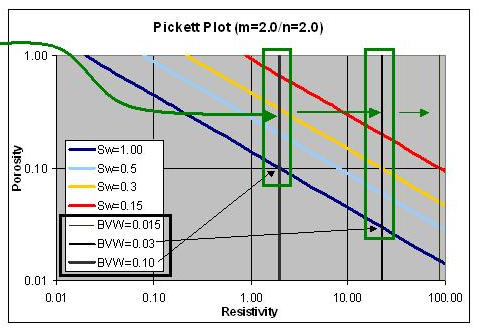
| FIG. 3
Double Duty
•
In the case of m = n, the porosity term [ (m - n)*Log
( Phi ) drops out leaving
Log(Rt) = Log(Rw) - n*Log(BVW)
= Constant
•BVW
= Constant grids are vertical
•BVW
lines below Sw = 100 % line are a mathematical extrapolation (for
visual reference) and not physically realistic
|
(m - n)*Log(Phi) = Log(Rw) - n*Log(BVW) - Log(Rt)
In the case of m = n,
the porosity term
drops out
leaving
Log(Rt) = Log(Rw) - n*Log(BVW)
= Constant
The BVW = Constant (single pore size) grids are vertical lines, on the Pickett Plot.
If
“m" and “n" are not equal, the
BVW grids are no longer vertical, as the porosity dependence in the above
relation does not drop out, but there remains a constraint, and a pattern, that
will appear on the Pickett Plot:
Figures 4 & 5.
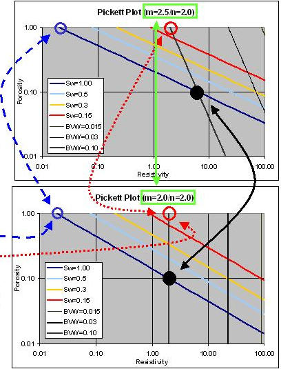
| FIG. 4
"m"
Not Equal to "n"
•
m=2.0 / n=2.0 vs m=2.5 / n=2.0
•‘m’
relates to pore system tortuosity, and as ‘m’ increases,
the resistivity of a specific porosity (10 pu in the graphic) at Sw
= 100 % also increases
•
Rw @ FT remains the same
•
Grids of constant BVW shift
•BVW
lines below Sw = 100 % are a mathematical extrapolation (for visual
reference) and not physically realistic
|
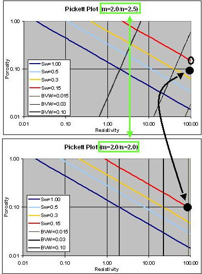
| FIG. 5
"m"
not Equal to "n"
•
m=2.0 / n=2.0 vs m=2.0 / n=2.5
•"n"
relates to the tortuosity of the conductive phase and as Sw
decreases the associated rise in resistivity of a specific porosity
is greater than what would have occurred at a lower
"n" value.
•Alternatively,
the Sw associated with a specific porosity & resistivity
increases as "n" increases.
|
Note that in some cases, this Double Duty situation could even allow one to deduce "m" from a water leg analysis, and "n" from the hydrocarbon zone response (actually "m - n", but with "m" known from the water leg, it will be possible to deduce "n" ).
The Old and The New
Although
the two (BVW and PP) concepts were once common, they are less commonly seen
today, than 30 years ago. In fact, during a recent course presentation I was
told that the Bulk Volume Water concept was only useful in ‘big Middle East
Fields’: even though the individual who made that statement was almost
certainly receiving NMR interpretations that included Bulk Volume Irreducible.
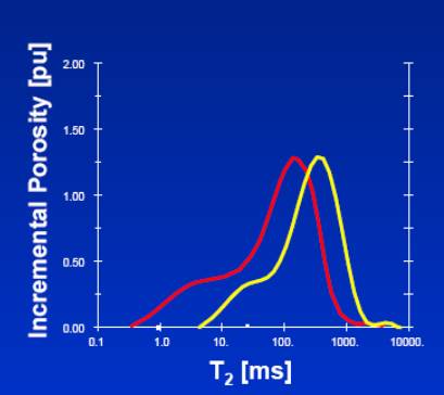
Today’s nuclear magnetic resonance measurements typically yield a mineral independent porosity and a pore size distribution (and potentially yet more): Figures 6 & 7.
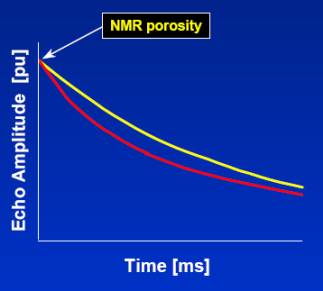
FIG. 6 Mineral
independent Porosity
| FIG. 6
•
Mineral Independent Porosity
•BVI
- Bulk Volume Irreducible water which includes water
retained by capillary forces in small pores, and water
wetting pore surfaces.
•BVM
- Bulk Volume Moveable, (Free Fluid Volume) which is porosity
available for hydrocarbon storage and fluid flow
|
- Yellow
Arrow : BWM ( Bulk Volume Moveable Water )
| FIG. 7
•
Mineral Independent Porosity
•BVI
- Bulk Volume Irreducible water
which includes water
retained by capillary forces in small pores,
and water wetting pore surfaces.
•BVM
- Bulk Volume Moveable, (Free
Fluid Volume) which is porosity
available for hydrocarbon storage and fluid flow.
|
The
NMR pore size distribution is often further characterized in
terms of Bulk Volume Irreducible; the fraction of the porosity expected
to be filled by capillary bound water, above the transition zone.
When Phi * Sw(Archie) ~ Bulk Volume Irreducible (NMR), water free
production can be anticipated, even if Sw is relatively high
(high capillary bound water).
On the other hand, low BVI (NMR) could signal water cut, even though Sw
(Archie) is relatively low (but greater than BVI (NMR)). Be aware that
specific cutoffs should be tailored to the reservoir / rock type in question.
In those cases for which we have conventional porosity
and resistivity logs, plus an NMR, it’s now
possible to combine The Old and The New, by annotating (in the
“z" direction) the Pickett Plot with NMR T2 results, thereby
compounding the value of the two perspectives.
Summary
With
today’s tool technology and computer power, it’s easy to over-look the
Tried And True Methods of Yester-Year. A better approach is to retain
the traditional methods (as appropriate) and build upon them with
today’s technology and computer power.
In addition to ensuring internal consistency of data / interpretations,
one could conceivably develop improved
evalualuation for legacy data which does not include the modern tools.
- Archie,
G. E. Classification of Carbonate Reservoir Rocks and Petrophysical
Considerations, AAPG Bulletin Vol 36 No 2 (1952): 278 - 296
- Aguilera,
Roberto, 1990, Extensions of Pickett plots for the analysis of shaly
formations by well logs: The Log Analyst, v. 31, no. 6, p. 304-313
- Aguilera,
Roberto , Incorporating capillary pressure, pore throat aperture radii,
height above free-water table, and Winland r35 values on Pickett
plots.
AAPG Bulletin, v. 86, no. 4 (April 2002), pp. 605–624
- Aguilera,
Roberto, Integration of geology, petrophysics, and reservoir engineering for
characterization of carbonate reservoirs through Pickett plots.
AAPG Bulletin, v. 88, no. 4 (April 2004), pp. 433–446
- Pickett,
G R, A Review of Current Techniques for Determination of Water
Saturation from Logs," paper SPE 1446, presented at the SPE Rocky
Mountain
Regional Meeting, Denver, Colorado, USA, May 23-24, 1966; SPE Journal of
Petroleum Technology (November 1966): 1425-1435.
THE COMPACT THEORY
DOWNLOAD
THE PDF FILE of the
DOUBLE_DUTY
NEWSLETTER COMPACT THEORY ----->
DOWNLOAD
GeoNeurale
Lichtenbergstrasse
8
85748 Munich-Garching
Germany
T +49 ( 0 ) 89 5484 0
T +49 ( 0 ) 89 5484 2240
T +49 ( 0 ) 89 89 69 1118
F +49 ( 0 ) 89 89 69 1117
www.GeoNeurale.com